")
目次
目的
カルマンフィルタの理論を学び直したくなった一環で、
1次元の車両位置を推定するという基本的なプログラムを
前回の記事で紹介しました。
www.eureka-moments-blog.com
今回はその応用として、1次元の車両位置に加えて速度を
線形カルマンフィルタで同時に推定するPythonプログラム
を作ったので紹介します。
問題設定
下図のように、ある速度で走行する車両の原点0からの
位置xと速度vを同時に推定することを考えます。
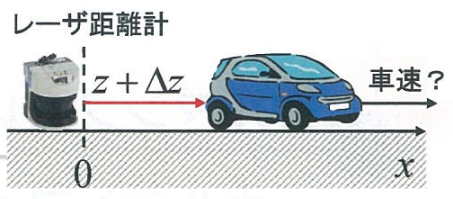
前回の問題と同様に、このときの車両の位置xは、
速度vより計算する方法と、レーザ距離計によりzとして
観測する方法の2つがあるとします。
また、車両が移動する間の速度vは、加速度aで
目標速度に達するまで変化し、目標速度に達して
からは一定となるものとします。
ただし、加速度aと観測zにはそれぞれ、分散Q, R
(平均値はともに0)の傾向を示す誤差が含まれます。
以上のような誤差分散を持つ加速度aと観測zを
利用して、カルマンフィルタにより車両の位置x,
速度v, 誤差共分散Pを推定することを本問題の
目的とします。
条件
- 目標速度vは10[m/s]、加速度aは5[m/s2]とする。
- 加速度aの持つ誤差分散Qは0.5とする。
- 観測zの持つ誤差分散Rは5.0とする。
Pythonプログラム
それではここからはプログラムの実装について
解説していきます。
パラメータの定義
まずは、今回のカルマンフィルタの計算に必要な
パラメータを下記のように定義します。
INTERVAL_SEC = 0.01
TIME_LIMIT_SEC = 10.0
TIME_LIMIT_ACCEL_SEC = 2.0
INPUT_ACCEL_MS2 = 5.0
INPUT_NOISE_VARIANCE = 0.5
OBSERVATION_NOISE_VARIANCE = 5.0
これらは上から順に、
- シミュレーションの刻み時間[秒]
- シミュレーションの実行時間[秒]
- 加速させる時間[秒]
- 加速度入力[m/s2]
- 加速度入力に含む誤差分散
- 観測値に含む誤差分散
となっています。
運動モデルクラスの定義
前回の記事でも書いたように、カルマンフィルタに
よる推定は、予測と更新という2つのステップに
分かれます。
そのため、運動モデルによって前時刻からの
車両位置と速度、そしてそれらの誤差共分散を
予測するためのパラメータとロジックを持つクラス
を定義することにします。
まずは、コンストラクタを下記のように実装します。
class MotionModel:
    """
    Class to predict 2 dimensional state (position and velocity) by Linear Motion Model
    """

    def __init__(self, interval_sec, input_noise_variance):
        """
        Constructor
        interval_sec: interval time[s] to update this simulation
        input_noise_variance: variance of noise included in input acceleration
        """

        # set inputs as parameters
        self.DT = interval_sec
        self.Q = np.array([[input_noise_variance]])

        self.define_matrix_in_state_equation()
コンストラクタでインスタンスを生成する際は、
パラメータとして定義したシミュレーションの
刻み時間と、加速度入力が含む誤差分散を
入力引数として与えるようにします。
また、プライベート関数として
define_matrix_in_state_equation()を定義し、
運動モデルとして用いる状態方程式に
含まれる行列F, Gを設定するようにします。
def define_matrix_in_state_equation(self):
    self.F = np.array([[1.0, self.DT],
                       [0.0, 1.0]])

    self.G = np.array([[(self.DT ** 2)/2],
                       [self.DT]])
詳しくはこちらの解説を参照していただきたい
のですが、Fはシステムの時間遷移に関する
線形モデル、Gは時間遷移に関する雑音モデルの
行列になります。
ja.wikipedia.org
続いて、上記のF, Gを用いた状態方程式を定義した
こちらの関数を定義し、車両位置と速度の予測に
用います。
def calculate_state(self, x_prev, u):
    """
    Function of state equation
    This is used to predict vehicle's position and velocity at next time
    by using acceleration input
    x_{t+1} = F * x_t + G * u_t

    x_prev: position and velocity at previous time, x_t
    u: acceleration input, u_t
    """

    x_next = self.F @ x_prev + self.G @ u
    return x_next
そして、システムの状態が含む誤差分散を
合わせて予測する関数も定義します。ちなみに、
今回のような問題では、車両位置の誤差と速度の
誤差という二組の対応するデータ間の関係を
表す分散である共分散を予測、推定することに
なります。
manabitimes.jp
観測モデルクラスの定義
次に、レーザ距離計の疑似的な観測値を生成する
ロジックと、運動モデルによって予測した時点に
得られる観測値を予測する観測方程式のロジックを
持つクラスを定義します。
コンストラクタはこちらのように定義します。
class ObservationModel:
    """
    Class to simulate position info obseved by LiDAR
    and to predict observation at predicted position, x_{t+1}
    """

    def __init__(self, observation_noise_variance):
        """
        Constructor
        observation_noise_variance: variance of noise included in observation
        """

        # set input as parameter
        self.R = np.array([[observation_noise_variance]])

        # define matrix in observation equation
        self.H = np.array([[1.0, 0.0]])
コンストラクタを生成する際の入力引数には、
事前にパラメータとして定義した観測誤差分散を
与えるようにします。また、観測方程式に
含まれるHも一緒に定義しています。
次に、疑似的な観測値を生成する関数を
下記のように定義します。
def observe(self, x_true):
    """
    Function to simulate observation by including noise variance
    parameter, R
    x_true: true position
    """

    return x_true[0, 0] + np.random.randn() * self.R
先に定義した運動モデルの状態方程式で
計算された車両の真の位置を入力で与え、
パラメータの観測誤差分散を持った正規分布
のノイズを付加するようにしています。
あとは観測方程式の関数も定義しておきます。
def calculate_observation(self, x_pred):
    """
    Function to predict observation at predicted position
    x_pred: predicted position by state equation, x_{t+1}
    """

    z_pred = self.H @ x_pred
    return z_pred
運動モデルで予測した状態を入力し、それを
Hにより観測値の予測に変換しています。
カルマンフィルタクラスの定義
最後に、ここまでに定義した運動モデルと
観測モデルのクラスを利用して、カルマン
フィルタによる状態推定を行うクラスを
定義します。
コンストラクタは下記のようになります。
ここまでに定義した運動モデルクラスと
観測モデルクラスのオブジェクトを引数
として渡すことでインスタンスを生成
します。
class LinearKalmanFilter2D:
    """
    Class to estimate 2 dimensional state (position and velocity) by Linear Kalman Filter
    """

    def __init__(self, motion_model, observation_model):
        """
        Constructor
        motion_model: motion model to predict state
        observation_model: model to predict observation at predicted position
        """

        self.mm = motion_model
        self.om = observation_model
ここからは、状態を推定するまでに必要な
ロジックを計算する関数を実装して
いきます。
まずは、観測値と予測値の誤差である
イノベーションを計算する関数です。
def calculate_innovation(self, z, x_pred):
    """
    Function to calculate innovation
    dz = z_{t+1} - H * x_{t+1}

    x_pred: predicted position with previous data, x_{t+1}
    """

    delta_z = z - self.om.calculate_observation(x_pred)
    return delta_z
続いて、観測予測誤差の共分散を計算する
関数を下記のように実装します。
def calculate_obsrv_pred_err_cov(self, p_pred):
    """
    Function to calculate observation prediction error variance
    s_{t+1} = H * p_{t+1} * H^T + R

    p_pred: predicted variance with previous data, p_{t+1}
    """

    p_obsrv_pred_err = self.om.H @ p_pred @ self.om.H.T + self.om.R
    return p_obsrv_pred_err
そして、ここまでに実装したロジックで
計算される状態の予測値と観測予測誤差の
共分散を使ってカルマンゲインを計算する
関数を下記のように実装します。
def calculate_kalman_gain(self, p_pred, p_obsrv_pred_err):
    """
    Function to calculate kalman gain
    k_{t+1} = p_{t+1} * H^T * s_{t+1}^{-1}

    p_pred: predicted variance with previous data, p_{t+1}
    p_obsrv_pred_err: observation prediction error variance, s_{t+1}
    """

    kalman_gain = p_pred @ self.om.H.T @ np.linalg.inv(p_obsrv_pred_err)
    return kalman_gain
前回の記事で扱ったような1次元の車両位置
のみを推定する問題と違い、今回のように
位置と速度を推定する問題では、共分散や
カルマンゲインがベクトルあるいは行列と
なるので、上記の関数内の計算では転置
行列や逆行列を扱うようになっています。
ここでの転置行列や逆行列の計算が何故
必要になるかはこちらの記事で導出して
いるので参照ください。
www.eureka-moments-blog.com
最後に、ここまでのロジックで計算される
状態の予測値、イノベーション、カルマンゲイン、
観測予測誤差の共分散を用いた状態の更新を
する関数と、誤差の共分散を更新する関数を
それぞれ下記のように実装します。
def calculate_state(self, x_pred, delta_z, kalman_gain):
    """
    Function to calculate position and velocity
    x^_{t+1} = x_{t+1} + k_{t+1} * dz

    x_pred: predicted position and velocity with previous data, x^_{t+1}
    delta_z: difference between observation and predicted observation, dz
    kalman_gain: kalman gain to update position and velocity, k_{t+1}
    """

    x_updated = x_pred + kalman_gain @ delta_z
    return x_updated

def calculate_covariance(self, p_pred, kalman_gain, p_obsrv_pred_err):
    """
    Function to calculate covariane of position and velocity
    p^_{t+1} = p_{t+1} - k_{t+1} * s_{t+1} * k_{t+1}^T

    p_pred: predicted covariance with previous data, p^_{t+1}
    kalman_gain: kalman gain to calculate position and velocity, k_{t+1}
    p_obsrv_pred_err: observation prediction error variance, s_{t+1}
    """

    p_updated = p_pred - kalman_gain @ p_obsrv_pred_err @ kalman_gain.T
    return p_updated
以上、ここまで実装してきた関数を一通り
組み合わせて、カルマンフィルタによる
一連の状態推定を行う関数を下記のように
実装します。
def estimate_state(self, x_prev, p_prev, u, z):
    """
    Function to estimate state and covariance by linear kalman filter
    Step 1: update state and covariance with previous data
    Step 2: update state and covariance with current observation

    x_prev: estimated state at previous time
    p_prev: estimated covariance at previous time
    u: acceleration input including gaussian noise
    z: observed position at current time including gaussian noise
    """

    # update with previous data
    x_pred = self.mm.calculate_state(x_prev, u)
    p_pred = self.mm.calculate_covariance(p_prev)

    # update with current observation
    delta_z = self.calculate_innovation(z, x_pred)
    p_obsrv_pred_err = self.calculate_obsrv_pred_err_cov(p_pred)
    kalman_gain = self.calculate_kalman_gain(p_pred, p_obsrv_pred_err)
    x_updated = self.calculate_state(x_pred, delta_z, kalman_gain)
    p_updated = self.calculate_covariance(p_pred, kalman_gain, p_obsrv_pred_err)

    return x_updated, p_updated
プログラムの実行結果
ここまでの実装により、今回の問題である
1次元の車両位置と速度をカルマンフィルタで
推定するシミュレーションができるように
なります。そのためのコード全体は下記の
ようになります。
def decide_input_accel(elapsed_time_sec):
    """
    Function to decide acceleration input
    Increasing velocity until time limit passed
    elapsed_time_sec: current elapsed time[sec]
    """

    if elapsed_time_sec <= TIME_LIMIT_ACCEL_SEC: input_accel_ms2 = INPUT_ACCEL_MS2
    else: input_accel_ms2 = 0.0

    return np.array([[input_accel_ms2]])


def add_noise_input_accel(input_accel_ms2):
    """
    Function to generate acceleration input
    including gaussian noise
    input_accel_ms2: true acceleration input
    """

    input_accel_noise_ms2 = input_accel_ms2[0, 0] + np.random.randn() * INPUT_NOISE_VARIANCE
    if input_accel_noise_ms2 < 0.0: input_accel_noise_ms2 = 0.0
    return np.array([[input_accel_noise_ms2]])


def main():
    """
    main function
    """

    print(__file__ + " start!!")

    # generate instances
    mm = MotionModel(interval_sec=INTERVAL_SEC, input_noise_variance=INPUT_NOISE_VARIANCE)
    om = ObservationModel(observation_noise_variance=OBSERVATION_NOISE_VARIANCE)
    kf = LinearKalmanFilter2D(motion_model=mm, observation_model=om)

    # initialize data
    input_accel_ms2 = 0.0
    elapsed_time_sec, time_list = 0.0, []
    true_state, true_pos_list, true_vel_list = np.zeros((2, 1)), [], []
    pred_state, pred_pos_list, pred_vel_list = np.zeros((2, 1)), [], []
    obsrv, obsrv_list = 0.0, []
    est_state = np.zeros((2, 1))
    est_cov = np.array([[OBSERVATION_NOISE_VARIANCE, 0.0],
                        [0.0, INPUT_NOISE_VARIANCE]])
    est_pos_list, est_vel_list, est_pos_cov_list, est_vel_cov_list = [], [], [], []

    # initialize plot
    fig = plt.figure()
    # position plot
    ax_position = fig.add_subplot(2, 2, 1)
    ax_position.set_xlabel("Time[s]")
    ax_position.set_ylabel("Position[m]")
    ax_position.grid(True)
    # position variance plot
    ax_pos_var = fig.add_subplot(2, 2, 2)
    ax_pos_var.set_xlabel("Time[s]")
    ax_pos_var.set_ylabel("Pos Var")
    ax_pos_var.grid(True)
    # velocity plot
    ax_veloicity = fig.add_subplot(2, 2, 3)
    ax_veloicity.set_xlabel("Time[s]")
    ax_veloicity.set_ylabel("Velocity[m/s]")
    ax_veloicity.grid(True)
    # velocity variance plot
    ax_vel_var = fig.add_subplot(2, 2, 4)
    ax_vel_var.set_xlabel("Time[s]")
    ax_vel_var.set_ylabel("Vel Var")
    ax_vel_var.grid(True)

    # simulate
    while TIME_LIMIT_SEC >= elapsed_time_sec:
        input_accel_ms2 = decide_input_accel(elapsed_time_sec=elapsed_time_sec)
        input_accel_noise_ms2 = add_noise_input_accel(input_accel_ms2)

        # calculate data
        obsrv = om.observe(true_state)
        true_state = mm.calculate_state(x_prev=true_state, u=input_accel_ms2)
        pred_state = mm.calculate_state(x_prev=pred_state, u=input_accel_noise_ms2)
        est_state, est_cov = kf.estimate_state(x_prev=est_state, p_prev=est_cov,
                                               u=input_accel_noise_ms2, z=obsrv)

        # record data
        time_list.append(elapsed_time_sec)
        obsrv_list.append(obsrv[0, 0])
        true_pos_list.append(true_state[0, 0]), true_vel_list.append(true_state[1, 0])
        pred_pos_list.append(pred_state[0, 0]), pred_vel_list.append(pred_state[1, 0])
        est_pos_list.append(est_state[0, 0]), est_vel_list.append(est_state[1, 0])
        est_pos_cov_list.append(est_cov[0, 0]), est_vel_cov_list.append(est_cov[1, 1])

        # increment time
        elapsed_time_sec += INTERVAL_SEC

    # plot data
    ax_position.plot(time_list, obsrv_list, color='g', lw=2, label="Observed Position")
    ax_position.plot(time_list, pred_pos_list, color='m', lw=2, label="Pred Position")
    ax_position.plot(time_list, true_pos_list, color='b', lw=2, label="True Position")
    ax_position.plot(time_list, est_pos_list, color='r', lw=2, label="Estimated Position")
    ax_position.legend()
    ax_veloicity.plot(time_list, pred_vel_list, color='m', lw=2, label="Pred Velocity")
    ax_veloicity.plot(time_list, true_vel_list, color='b', lw=2, label="True Velocity")
    ax_veloicity.plot(time_list, est_vel_list, color='r', lw=2, label="Estimated Velocity")
    ax_veloicity.legend()
    ax_pos_var.plot(time_list, est_pos_cov_list, color='r', lw=2, label="Est Pos Variance")
    ax_pos_var.legend()
    ax_vel_var.plot(time_list, est_vel_cov_list, color='r', lw=2, label="Est Vel Variance")
    ax_vel_var.legend()
    fig.tight_layout()

    # only when show plot flag is true, show output graph
    # when unit test is executed, this flag become false
    # and the graph is not shown
    if show_plot: plt.show()

    return True
これを実行すると、こちらのような結果が
得られます。
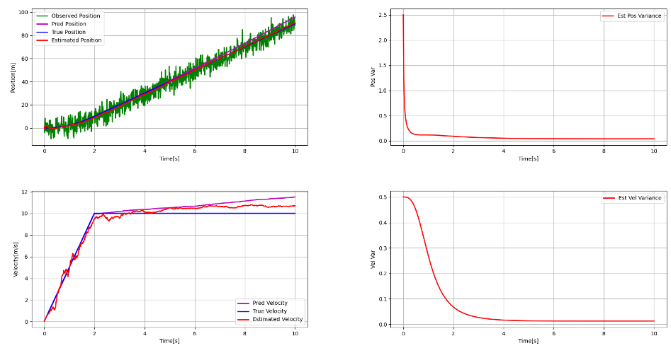
左上段のグラフが車両位置の推定結果ですが、
緑が観測値、青が真値、紫は予測値、赤が
カルマンフィルタによる推定値です。
また、左下段のグラフが車両速度の推定結果であり、
青が真値、紫は予測値、赤が推定値です。
どちらの場合においても、予測だけでは誤差が
蓄積されて真値からどんどん離れてしまっており、
カルマンフィルタの推定なら真値に近い値と
なっていることがわかります。
右側の上下のグラフはそれぞれ位置と速度の
誤差分散の推定位置であり、これらが小さく
なっていくような高精度な推定ができている
ことがわかります。
以上、ここまでで、1次元の車両位置と速度を
推定できるカルマンフィルタを実装することが
できました。
GitHub
今回紹介したPythonプログラムは、こちらの
GitHubリポジトリでも公開しています。
github.com