Fundamentals of Regression by Machine Learning

Table of contents

Introduction

This is my studying log about machine learning, regression. I referred to a following book.

Pythonで動かして学ぶ!あたらしい機械学習の教科書 第2版

I extracted some important points and some related sample python codes and wrote them as memo in this article.

Author

Makoto Ito

GitHub

Sample codes for plotting the following figures are released at my GitHub repository.

github.com

Linear model with 1 dimensional input

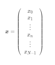
Input data: Age

Target data: Height

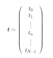
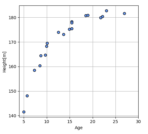
N means the number of people and N = 20. A purpose of this regression is predicting a height with an age of a person who is not included the databases.

Data generation

Linear model definition

• Linear equation:
  

• Mean squared error function:
  

• plot relationship between w and J:
  

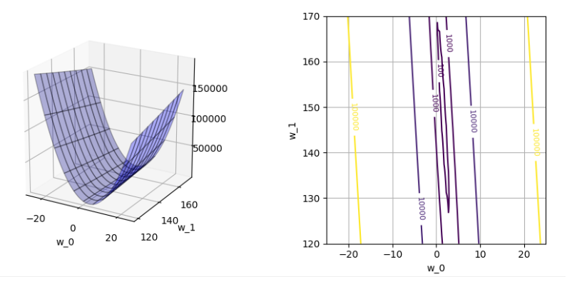
We need to decide w_0 and w_1 which minimize mean squared error, J. Depend on the above graph, J has a shape like a valley. And then, the value of J is changing to the direction of w_0, w_1. When w_0 is about 3 and w_1 is about 135, J will be minimized.

Gradient method

Gradient method is used for calculating w_0 and w_1 which minimize the value of J. This method repeat the following calculation:

1. Select a initial point, w_0 and w_1 on the valley of J.
2. calculate a gradient at the selected point.
3. w_0 and w_1 are moved to the direction which the value of J most decline.
4. Finally, w_0 and w_1 will reach values which minimize the value of J.

Gradient to the going up direction:

Gradient to the going down direction:

Learning algorithm:

α is a positive number and called "Learning rate" which can adjust a update width of w. The bigger this number is, the bigger the update width is, but a convergence of calculation will be unstable.

Learning Result

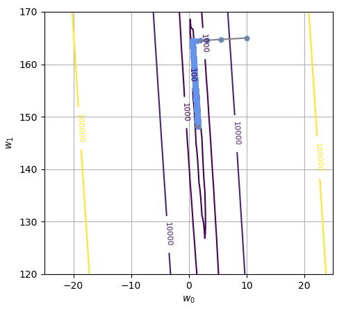
• Learning behavior plot:
  Initial point: [10.0, 165.0]
  Final point: [1.598, 148.172]
  Number of iteration: 12804
  

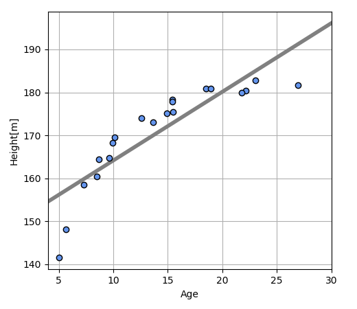
• Predicted linear line plot:
  Mean squared error: 29.936629[cm²]
  Standard deviation: 5.471[cm]
  

Point to notice

The result which is solved by Gradient method is just a local minimum value and not always global minimum value. Practically, we need to try gradient method with various initial values and select the minimum result value.

Plane model with 2 dimensional input

In this case, data vector xx is extended to 2 dimensional data, (x_0, x_1). x_0 is age and x_1 is weight.

Data generation

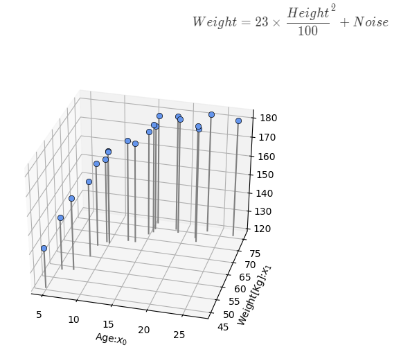
Plane model

• Definition of surface function:
  
• Mean squared error function:
  
• Gradient:
  
• Optimal parameters:
  
• Learning result:
  

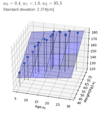
D-dimensional Linear Regression Model

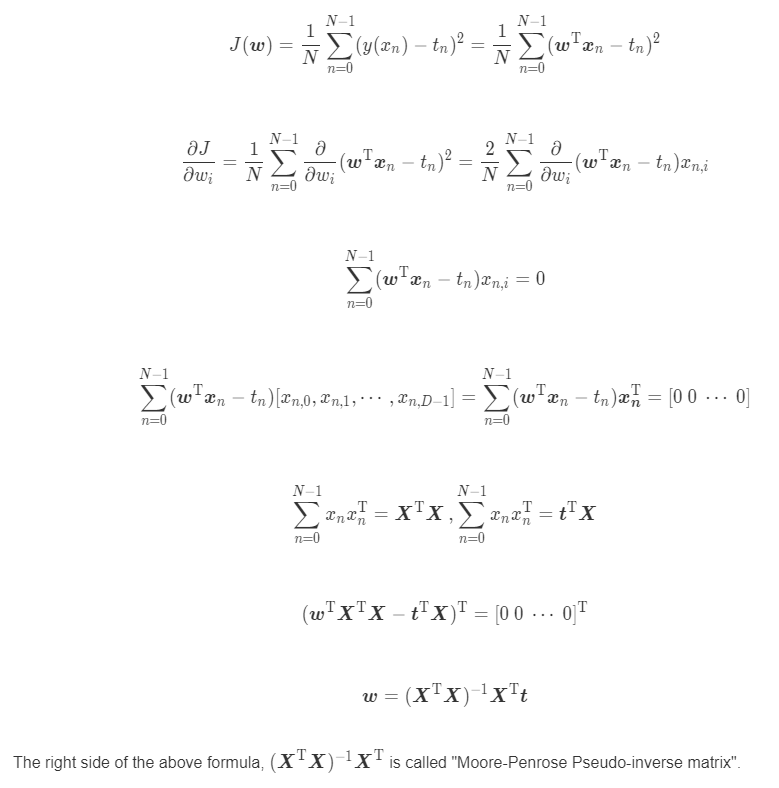
• It requires a lot of work to derive all of formulas at different dimension. So, we need to define the number of dimension as a variable, D.

• We can shorten the above model with Matrix representation.

Solution of model

Extension to plane not passing through origin

Vector x can be thought as 3 dimensional vector by adding 3rd element which is always "1". In case that x_2 =1.

Linear basis function

• Way of thinking

x of Linear Regression model is replaced with Basis function ϕ(x) to create a function which has various shapes.

• Gaussian function

Gaussian function is used as basis function in this section. Basis function is used as multiple sets and a suffix j is attached in the formula. s is a parameter to adjust a spread of the function.

• Combined function M gaussian functions

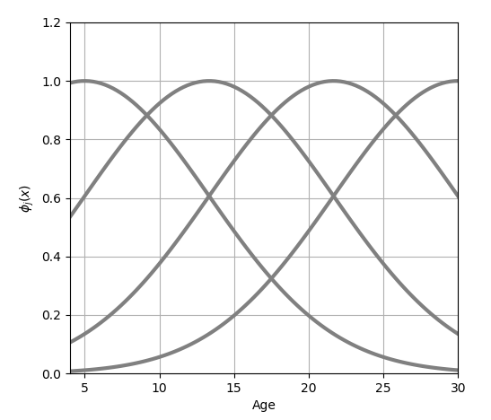
M is the number of combined functions. In the above, M=4
Weight parameters for each function: w_0, w_1, w_2 , w_3
A parameter for adjusting up and down movement of model: w_4
w_4 is for a dummy function, ϕ_4​(x)=1.

• Mean squared error J

• Solution w

• Preprocessed input data ϕ

ϕ is called "Design matrix".

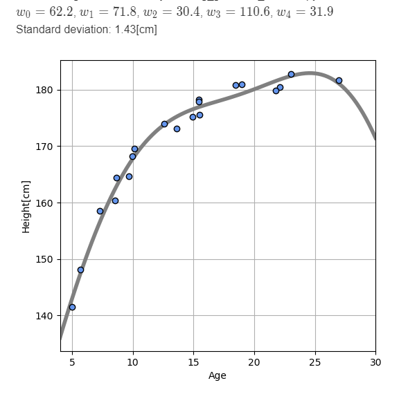
• Learning Result

Overfitting problem

Standard deviation of error is decreasing by increasing the number of M but, the basis function is getting more curved as follow.

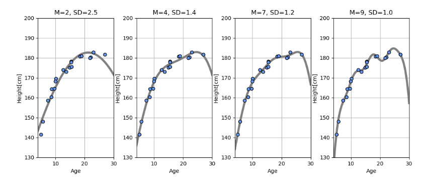
This curve gets close to each sample points but it becomes deformed at a part where there is no sample point. This is called "over-fitting". The prediction for a new data will become bad.

Hold-out validation

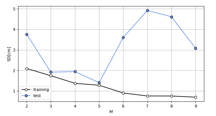
All of data, x and t are divided into "Test data" and "Training data". For this example, 1/4 of data is used for test and the rest, 3/4 is used for training. The parameter of model, w is optimized with only training data and a mean squared error for test data is calculated with the optimized parameter w.

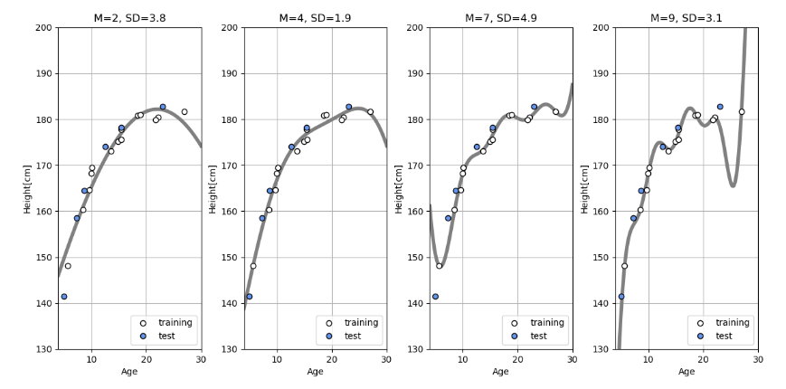
In the above graphs, white points are training data and blue points are test data. If the number of M is over than 4, standard deviation for test data gets worth and over-fitting occurs.

Cross-validation

The above result depends on how to select training data. This dependency is revealed prominently when the number of data is a few.

K-hold cross-validation

Data X and t are divided into K groups. One of them is used for test and the rest is used for training. Calculating parameters of model and mean squared error is executed for K times, and then an average of mean squared error for K times is calculated. The average value is used for validating the parameters of model.

Leave-one-out cross-validation

A maximum number of division is K=N. In this case, a size of test data is 1. This method is called "leave-one-out cross-validation".

Validation result

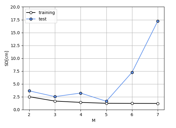
This is a difference of standard deviation depending on M. When M is 5, the standard deviation is smallest. When a size of data is small, cross-validation is useful. The larger the size of data is, the longer time it takes to calculate the validation.

Model improvement

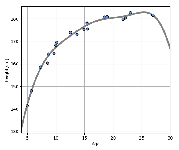
The above model still has a problem. It is that the graph is descending at over than 25 years old. This tendency is unusual.

Correct tendency

Height will increase gradually with age and converge at a certain age.

New model

Each parameter, w_0, w_1, w_2 is a positive number. exp(-w_2 x)exp will close to 0 when xx increase. w_0 is a convergence value. w_1 is a parameter to decide a start point of the graph. w_2 is a parameter to decide a slope.

Optimization

The above parameters w is calculated by resolving optimization problem with scipy library.

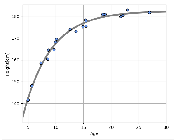
These optimized parameters w_0=182.3, w_1=107.2, w_2=0.2. Standard deviation of error is 1.31[cm].

Model selection

I need to select the best model by comparing their prediction accuracy. The following model A and B are compared by leave-one-out cross-validation.

Model A

Model B

Comparison result

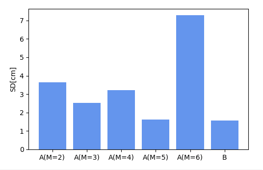
• Standard deviation(Model A): 1.63[cm]
• Standard deviation(Model B): 1.55[cm]
  According to this validation, I can conclude that Model B is more suitable to the data than Model A.

Conclusion

This is a flow of data analysis(model selection) by supervised learning.

1. We have data: input valuables and target valuables.
2. Purpose function is decided. This function is used for judging a prediction accuracy.
3. Candidates of model are decided.
4. If we choose hold out validation as a validation method, we need to divide all of data into training data and test data.
5. A parameter of each model is decided with training data in minimizing or maximizing the purpose function.
6. We predict target data from input data by each model with decided parameters and the model which the error is the smallest.